Loading [MathJax]/jax/output/CommonHTML/fonts/TeX/fontdata.js

Assessment of the surface area of a sphere

A sphere is a common geometrical object of choice in many computational sciences used to approximate continuous, closed surfaces forming 3-D ball-like models. Concretely, in my research area - computational bioelectromagnetics and dosimetry, or in computational neuroscience for example, we often approximate the surface of the human head by using a sphere.

Even though this kind of representation of real world objects is a crude geometrical approximation, see Fig. 1 below, it allows a much simpler simulation setup due to the high symmetry of the solution domain.

Figure 1. This would have been Mona Liza had Leonardo da Vinci been a computational scientist. Jokes aside, this painting is the work by the great Fernando Botero, a Colombian figurative artist and sculptor whose signature style often depicts people and figures in hyperbolic manner.

One of the common issues in simulations is the estimation of the total surface area of a portion of the observed object. For regular spherical surfaces, this is fairly easy to do, and yet in this short essay, I will demonstrate the hard way to do it.

Let's start by calculating the area of a sphere defined by some radius, $r$, using the following closed-form expression:

$$A = 4 \pi r^2$$

from scipy.constants import pi


r = 1.
A_analytic = 4 * pi * r ** 2
print(f'A = {A_analytic:.6f}')

A = 12.566371

It turns out that the area of a sphere with a radius set to $1$ amounts to $\sim12.566361$.

The closed-form expression derives from the surface integral of a tiny surface element, $dA$, on the sphere, in spherical coordinates given as:

$$dA = r^2 \sin \theta d\theta d\phi$$

More details on the parametrization should be found elsewhere, e.g., in this very short video lecture by Khan Academy.

The overall area is obtained by integrating all these tiny surface elements for the entire domain, $\theta \in [0, 2\pi]$ and $\phi \in [0, \pi]$, and by setting the radius to a fixed value:

$$A = \int_{0}^{2\pi}\int_{0}^{\pi}r^2 \sin \theta d\theta d\phi$$

There is no chance I will do the math by hand. I am not even sure if I know how to. I am not even sure if I own a pen and paper anymore... Rather, let's take advantage a very smart box called computer and implement Gauss quadrature, introduction of which is available on Wikipedia. In a nutshell, the above integral can be approximated as a weighted sum of each surface element at each specific point within the domain. These "specific" points, and associated weights, arise from the choice of underlying polynomials that define our domain. Here, we are going to use Legendre polynomials.

import numpy as np


# define `theta` and `phi`, and set `r` to 1
theta = (0., pi)
phi = (0., 2 * pi)
r = 1.

# extract and scale roots and weights for quadrature using Legendre polynomials
deg = 20
roots, weights = np.polynomial.legendre.leggauss(deg)
theta_roots = 0.5 * (roots + 1.) * (theta[1] - theta[0]) + theta[0]
theta_weights = 0.5 * weights * (theta[1] - theta[0])
phi_roots = 0.5 * (roots + 1.) * (phi[1] - phi[0]) + phi[0]
phi_weights = 0.5 * weights * (phi[1] - phi[0])
theta_grid, phi_grid = np.meshgrid(theta_roots, phi_roots)

# quadrature
A_quad = phi_weights @ np.sin(theta_grid) * r ** 2 @ theta_weights
print(f'A = {A_quad:.6f}')

A = 12.566371

Nice, we are accurate to at least the 6th decimal, which should be satisfactory for most small-scale applications.

However, the main issue with this approach is that we have to use predefined set of sample points and weights. In real-world applications and simulations, points are unordered, random, sometimes even noisy. For irregular point clouds, we should first reconstruct the surface, and only then we can estimate the total surface area.

A common way to approach this issue, assuming that the surface is convex, is by triangulatng the surface by using the convex hull or envelope. The convex hull is the smallest convex region contating the point set which we have at our disposal, where this region is any region in which each point-pair is visible within the region itself. Important caveat is that convex hull algorithms suffer greatly, and result with invalid reconstructed regions for that matter, if there exist any kind of degenerate situations.

Now, let's first randomly generate a point cloud representing the sphere with the radius set to 1. For this, we will use the elegant method that consists of picking two values from independent uniform distributions, $a$ and $b$, and rejecting points that does not satisfy the following condition:

$$a^2 + b^2 \leq r$$

where $r$ stands for the radius of a ball.

After, the randomly generated point cloud is forwarded to scipy.spatial.ConvexHull class, and the surface area is simply obtained by accessing the attribute scipy.spatial.ConvexHull.area.

import matplotlib.pyplot as plt
from mpl_toolkits.mplot3d.art3d import Poly3DCollection
%config InlineBackend.figure_format = 'retina'
import scipy.spatial as ss


def marsaglia(n_points, r=1.):
    """Return a randomly generated point cloud representing a sphere.
    For implementation details visit:
    https://mathworld.wolfram.com/SpherePointPicking.html
    
    Refs: Marsaglia, G., Ann. Math. Stat. 43:645-646, 1972
    
    Parameters
    ----------
    n_points : int
        Proposed number of points of a sphere.
    r : float, optional
        Radius.
    
    Returns
    -------
    numpy.ndarray
        Set of points representing a sphere.
    """
    assert r > 0, 'radius must be a positive number'
    a = np.random.uniform(-r, r, size=n_points)
    b = np.random.uniform(-r, r, size=n_points)

    mask = np.where(a ** 2 + b ** 2 < 1)
    a = a[mask]
    b = b[mask]

    x = 2 * a * np.sqrt(1 - a ** 2 - b ** 2)
    y = 2 * b * np.sqrt(1 - a ** 2 - b ** 2)
    z = 1 - 2 * (a ** 2 + b ** 2)
    return np.stack((x, y, z), axis=-1)


# generate random point cloud
xyz = marsaglia(deg ** 2, r)

# create convex hull and extract the surface area
hull = ss.ConvexHull(xyz)
A_hull = hull.area
print(f'A = {A_hull:.6f}')

# visualize the randomly generated point cloud and reconstructed surface
fig = plt.figure(figsize=(6, 6))
ax = plt.axes(projection ='3d')
ax.scatter(*xyz.T, ec='k', c='None')
hull_triangle_coords = hull.points[hull.simplices]
triangles = Poly3DCollection(hull_triangle_coords, ec='k', lw=0.2, alpha=0.2)
ax.add_collection3d(triangles)
ax.set(xlabel='x', ylabel='y', zlabel='z',
       xlim=(-1, 1), ylim=(-1, 1), zlim=(-1, 1))
ax.view_init(20, -60)
fig.tight_layout();

A = 12.342118

Results are not as good as with the Gaussian-Legendre quadrature approach, but this is expected since a convex hull is nothing but a bunch of small planar polygons that reconstruct a sphere, and the sphere is inherently non-planar.

This problem can be somewhat circumvented if we generate a larger number of surface points. For example, if we set n_points argument of marsaglia function to $20000$ for example, we get a much, much better surface area estimate.

# generate random point cloud
xyz = marsaglia(20000, r)

# create convex hull and extract the surface area
hull2 = ss.ConvexHull(xyz)
A_hull2 = hull2.area
print(f'A = {A_hull2:.6f}')

A = 12.561579

Very nice.

All this so far is very nice, simple and elegant, but I want something that is a complete opposite of that. I will now demonstrate how to compute the area of a sphere in an overly complicated way just because I want to be a cool kid who uses new fancy libraries for sport.

Here, we are going to use jax and its automatic differentiation capabilities to extract the gradients of vectors normal to the sphere in order to compute the following integral, and thus estimate the surface area:

$$A = \int_x \int_y \sqrt{\Big(\frac{\partial z}{\partial x}\Big)^2 + \Big(\frac{\partial z}{\partial y}\Big)^2 + 1} dx dy$$

What is this integral anyway?

Well, we first have to set one of the coordinates, in this case I have chosen $z$, to be a function of other two:

$$z = z(x, y)$$

Since we talk about a sphere here, $z$, as a function of $x$ and $y$, is defined as:

$$z = z(x, y) = \pm \sqrt{r - x^2 - y^2}$$

where $r$, as always, stands for the radius.

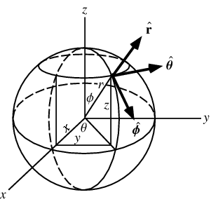
This parametrization yields the definition of the position vector $\vec r$, shown in Fig. 2, written as follows:

$$\vec r = \vec r(x, y) = x \vec i + y \vec j + z(x, y) \vec k$$

Figure 2. The position vector connects each point of a sphere to the ball origin. Image source: https://mathworld.wolfram.com/SphericalCoordinates.html

The magnitude of the cross product of the partial derivatives of $\vec r(x, y)$ yields the vector surface element, $\vec{dA}$:

$$\vec{dA} = \Big|\frac{\partial \vec r(x, y)}{\partial x} \times \frac{\partial \vec r(x, y)}{\partial y}\Big|$$

By following the defintion of the position vector, the partial derivatives with respect to $x$ and $y$ are respectively written as:

$$\frac{\partial \vec r}{\partial x} = \vec i + \frac{\partial z(x,y)}{\partial x} \vec k$$

and

$$\frac{\partial \vec r}{\partial y} = \vec j + \frac{\partial z(x,y)}{\partial y} \vec k$$

From here, it follows that

$$\vec{dA} = \Big|\Big(\vec i + \frac{\partial z(x,y)}{\partial x} \vec k \Big) \times \Big(\vec j + \frac{\partial z(x,y)}{\partial y} \vec k\Big)\Big| = \Big|\Big(-\frac{\partial z(x, y)}{\partial x}, -\frac{\partial z(x, y)}{\partial x}, 1\Big)\Big|$$

Finally, once we define the magnitude of this expression:

$$|\vec{dA}| = \sqrt{\Big(\frac{\partial z}{\partial x}\Big)^2 + \Big(\frac{\partial z}{\partial y}\Big)^2 + 1}$$

we finally have the reasoning behind the above mentioned surface integral.

The expression for $|\vec{dA}|$ can be separated in a following way:

$$|\vec{dA}| = dA \cdot \vec n$$

where $\vec n$ is the vector normal to the parameterized surface element $dA = dxdy$.

Okay, so entire outlined math here basically means that if we can somehow are able to compute gradients of the normal vector in each point on our parameterized surface, we can compute the overall surface area. The parametrization of a sphere is a bit tricky for a computer to handle it because it includes square roots, so instead parametrization of an entire sphere, we are going to parametrize only a small positive portion and scale the final area estimate accordingly. Let's begin.

from jax import (jit, grad, vmap)
import jax.numpy as jnp


# explicit sphere parametrization via z=z(x, y)
z_fn = lambda x, y, r: jnp.sqrt(r ** 2 - x ** 2 - y ** 2)


# derivatives of z(x,y) with respect to x and y
grad_z_fn = grad(z_fn, argnums=(0, 1))


# vectorized implementation of the above function
grad_z_fn_vmap = vmap(grad_z_fn, in_axes=(0, 0, None))


# define the domain using a polar coordinates...
u = (0, 1)
v = (0, np.pi)

roots, _ = np.polynomial.chebyshev.chebgauss(deg)
u_roots = 0.5 * (roots + 1.) * (u[1] - u[0]) + u[0]
v_roots = 0.5 * (roots + 1.) * (v[1] - v[0]) + v[0]

U, V = np.meshgrid(u_roots, v_roots)
X = U * np.sin(V)
Y = U * np.cos(V)
Z = z_fn(X, Y, r)

# compute the normal vector length in each point of interest
dzdx, dzdy = grad_z_fn_vmap(X.ravel(), Y.ravel(), r)
n_abs = np.sqrt(dzdx ** 2 + dzdy ** 2 + 1)

# compute unit vnormal vectors and orient them consistent to a tangent plane
nx = -dzdx / n_abs
ny = -dzdy / n_abs
nz = np.ones_like(nx) / n_abs

# integrate and scale the integral according to the definition of the domain
A_n = 4 * np.sum(n_abs[deg:] * (np.diff(X, axis=0).ravel() 
                                * np.diff(Y, axis=1).ravel()))
print(f'A = {A_n:.6f}')

# visualize the stuff we just did
fig = plt.figure(figsize=(6, 6))
ax = plt.axes(projection ='3d')
ax.scatter(X.ravel(), Y.ravel(), Z.ravel(), ec='k', c='None')
ax.quiver(X.ravel(), Y.ravel(), Z.ravel(),
          nx, ny, nz,
          length=0.3, lw=1, color='k')
ax.set(xlabel='x', ylabel='y', zlabel='z',
       xlim=(-1, 1), ylim=(-1, 1), zlim=(-1, 1))
ax.view_init(20)
fig.tight_layout();

WARNING:absl:No GPU/TPU found, falling back to CPU. (Set TF_CPP_MIN_LOG_LEVEL=0 and rerun for more info.)

A = 12.403081

Alright, not bad at all!

We managed to get pretty close to the actual value of the surface area. To wrap things up, let's generate a summary table of the results obtained via 3 different numerical tecniques in comparisson to the actual target value.

header = 'Method of choice  |  Computed value  |  Relative error'
print(header)
print('-' * len(header), sep='')
print(f'Analytical\t\t{A_analytic:.6f}\t'
      f'{np.linalg.norm(A_analytic - A_analytic) / A_analytic:.6e}')
print(f'Gauss-Legendre\t\t{A_quad:.6f}\t'
      f'{np.linalg.norm(A_analytic - A_quad) / A_analytic:.6e}')
print(f'Convex-Hull\t\t{A_hull:.6f}\t'
      f'{np.linalg.norm(A_analytic - A_hull) / A_analytic:.6e}')
print(f'Normal estim\t\t{A_n:.6f}\t'
      f'{np.linalg.norm(A_analytic - A_n) / A_analytic:.6e}')

Method of choice  |  Computed value  |  Relative error
------------------------------------------------------
Analytical		12.566371	0.000000e+00
Gauss-Legendre		12.566371	8.481479e-16
Convex-Hull		12.342118	1.784542e-02
Normal estim		12.403081	1.299419e-02